weatheR

This package contains a set of functions to download, transform, and plot data from NOAA ISD weather stations.

For example, you may want to:

Find the k-nearest stations to a city, or any other location that can be found via google maps
Plot the stations and reference point for any location
Download all k-nearest station data to a given location for a range of years
Select a station with the best data to a given location and interpolate missing observations

Installing via GitHub

require(devtools)
install_github("mpiccirilli/weatheR")
require(weatheR)

List of Weather Stations

The list of stations will be called in under the name station.list. The alternative is to use the function to call in the data.

data(stations)
# or
station.list <- allStations()

Now we can create a vector of cities we would like to download weather data. In order to search for stations by city, we need to use the following format: “city, country” or “city, state”.

cities <- c("Nairobi, Kenya", "Tema, Ghana", "Accra, Ghana", "Abidjan, Ivory Coast")

kNStations

This function will find the k-nearest weather stations to a given city. It is used all the functions to find stations.

k.n.stations <- kNStations(cities, station.list, 5)

plotStations

Before we download the data, we can inspect the cities to make sure there are in fact stations close to each city. If some of the stations are too far outside the area of the plot, you might receive a warning message indicating that some points have been excluded. As you can see, this occurs below.

The following function plots the k-nearest weather stations to a city’s reference point. The black dots are the reference points, and the red dots are the stations, ordered from 1 to k by closeness. I have included k in the function, however it is an optional parameter that will default to 5 if omitted.

plotStations(cities, station.list, 5)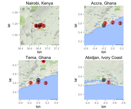

cityPlot

Now let’s download the station data.

In addition to the list of stations and cities, we have also included several other parameters to help us select the best station between a given date range. The parameters include:

k-nearst stations we would like to select (optional; default=5)
beginning date (required; 4-digit year)
end date (required; 4-digit year)
max distance in kilometers away from a location to consider (optional; default=100)
minimum hourly interval of observations. ex, 1 = hourly, 3 = every three hours, etc.. (optional; default=3)
tolerance, which ismax percent of missing data we will allow (optional; default=.05)
As you will see in the examples below, I do not include the optional parameters except in getInterpolatedDataByCity.

getStationsByCity

This function will downlaod each year of data for the k-nearest stations (default = 5) for each city, so it will take some time to run. The output of the function is a list of two:

dl_status: This is the status of attempting to download each year of each station.
station_data: This is a list of dataframes with the station data

stations <- getStationsByCity(cities, station.list, begin = 2012, end = 2013)

stations$dl_status

##                   File  Status                 City rank kilo_distance
##   655780-99999-2012.gz Success Abidjan, Ivory Coast    1     13.396883
##   655780-99999-2013.gz Success Abidjan, Ivory Coast    1     13.396883
##   655850-99999-2012.gz Success Abidjan, Ivory Coast    2     81.198627
##   655850-99999-2013.gz Success Abidjan, Ivory Coast    2     81.198627
##   655620-99999-2012.gz Success Abidjan, Ivory Coast    3    165.546591
##   655620-99999-2013.gz Success Abidjan, Ivory Coast    3    165.546591
##   654650-99999-2012.gz Success Abidjan, Ivory Coast    4    205.531045
##   654650-99999-2013.gz Success Abidjan, Ivory Coast    4    205.531045
##   654450-99999-2012.gz Success Abidjan, Ivory Coast    5    212.170762
##   654450-99999-2013.gz Success Abidjan, Ivory Coast    5    212.170762
##   654720-99999-2012.gz Success         Accra, Ghana    1      7.121795
##   654720-99999-2013.gz Success         Accra, Ghana    1      7.121795
##   654730-99999-2012.gz Success         Accra, Ghana    2     23.349153
##   654730-99999-2013.gz Success         Accra, Ghana    2     23.349153
##   654490-99999-2012.gz  Failed         Accra, Ghana    3     40.986341
##   654490-99999-2013.gz  Failed         Accra, Ghana    3     40.986341
##   654590-99999-2012.gz Success         Accra, Ghana    4     59.512919
##   654590-99999-2013.gz Success         Accra, Ghana    4     59.512919
##   654710-99999-2012.gz  Failed         Accra, Ghana    5     68.850839
##   654710-99999-2013.gz  Failed         Accra, Ghana    5     68.850839
##   637420-99999-2012.gz Success       Nairobi, Kenya    1      3.416254
##   637420-99999-2013.gz Success       Nairobi, Kenya    1      3.416254
##   637390-99999-2012.gz Success       Nairobi, Kenya    2      4.756458
##   637390-99999-2013.gz Success       Nairobi, Kenya    2      4.756458
##   637410-99999-2012.gz Success       Nairobi, Kenya    3      8.044960
##   637410-99999-2013.gz Success       Nairobi, Kenya    3      8.044960
##   637403-99999-2012.gz  Failed       Nairobi, Kenya    4      8.044960
##   637403-99999-2013.gz  Failed       Nairobi, Kenya    4      8.044960
##   692014-99999-2012.gz Success       Nairobi, Kenya    5     10.601511
##   692014-99999-2013.gz Success       Nairobi, Kenya    5     10.601511
##   654730-99999-2012.gz Success          Tema, Ghana    1      5.521650
##   654730-99999-2013.gz Success          Tema, Ghana    1      5.521650
##   654720-99999-2012.gz Success          Tema, Ghana    2     19.707146
##   654720-99999-2013.gz Success          Tema, Ghana    2     19.707146
##   654490-99999-2012.gz  Failed          Tema, Ghana    3     19.907417
##   654490-99999-2013.gz  Failed          Tema, Ghana    3     19.907417
##   654710-99999-2012.gz  Failed          Tema, Ghana    4     48.059678
##   654710-99999-2013.gz  Failed          Tema, Ghana    4     48.059678
##   654600-99999-2012.gz Success          Tema, Ghana    5     49.882386
##   654600-99999-2013.gz Success          Tema, Ghana    5     49.882386

class(stations$station_data)
##  [1] "list"
length(stations$station_data)
##  [1] 15

getFilteredStationsByCity

This function is similar to getStationsByCity except this goes one more step and applies some filters to each of the stations so that we can select the ‘best’ station for each city. So this will return only 1 station per city, instead of the k-nearest available stations.

The output of the function is a list of four:

dl_status: This is the status of attempting to download each year of each station.
removed_rows: This shows the number of stations found, removed, and kept through the filtering process. The name comes from the filtering techniques used, which are based on the number of missing observations
station_names_final: the names of each dataframe in station_data. The format is: “city_USAFID”
station_data: This is a list of dataframes with the station data

stations <- getFilteredStationsByCity(cities, station.list, begin = 2012, end = 2013)

stations$dl_status  #same results as above

stations$removed_rows

##      city stations removed kept
##   Abidjan        5       3    2
##     Accra        3       2    1
##   Nairobi        4       1    3
##      Tema        3       2    1

stations$station_names_final
##  [1] "Abidjan_655780" "Accra_654720"   "Nairobi_637420" "Tema_654720" 


class(stations$station_data)
##  [1] "list"
length(stations$station_data)
##  [1] 4

getInterpolatedDataByCity

This function uses the same filtering procedure as getFilteredStationsByCity stations, selecting the best station for each city based on the number of missing observations and proximity to each city’s reference point. It will then average the hourly observations and interpolate any missing values.

The output of the function is a list of five:

dl_status: This is the status of attempting to download each year of each station.
removed_rows: This shows the number of stations found, removed, and kept through the filtering process. The name comes from the filtering techniques used, which are based on the number of missing observations
station_names_final: the names of each dataframe in station_data. The format is: “city_USAFID”
interpolated: This shows the number and percent of values that have been interpolated for each station
station_data: This is one large dataframe with all station data combined

To do:
1/24: Include optionality to return station_data as either a list or a dataframe

hourly.data <- getInterpolatedDataByCity(cities, station.list, 5, 2010, 2013, 100, 3, .05)

hourly.data$dl_status    # same results as above

hourly.data$removed_rows    # same results as above

hourly.data$station_names_final    # same results as above

hourly.data$interpolated
##                 num_interpolated pct_interpolated
##  Abidjan_655780              504       0.01437372
##  Accra_654720               7822       0.22307780
##  Nairobi_637420            17876       0.50981063
##  Tema_654720                8384       0.23910564


unique(hourly.data$station_data$city)
##  [1] "Abidjan" "Accra"   "Nairobi" "Tema"   

head(hourly.data$station_data)
##                 hours    city USAFID distance rank   YR M D HR  LAT   LONG ELEV  TEMP DEW.POINT
##   2010-01-01 00:00:00 Abidjan 655780 13.39947    1 2010 1 1  0 5.25 -3.933    8 27.50      26.5
##   2010-01-01 01:00:00 Abidjan 655780 13.39947    1 2010 1 1  1 5.25 -3.933    8 28.00      27.0
##   2010-01-01 02:00:00 Abidjan 655780 13.39947    1 2010 1 1  2 5.25 -3.933    8 28.00      28.0
##   2010-01-01 03:00:00 Abidjan 655780 13.39947    1 2010 1 1  3 5.25 -3.933    8 27.65      26.3
##   2010-01-01 04:00:00 Abidjan 655780 13.39947    1 2010 1 1  4 5.25 -3.933    8 28.00      26.0
##   2010-01-01 05:00:00 Abidjan 655780 13.39947    1 2010 1 1  5 5.25 -3.933    8 27.00      26.0

plotDailyMax

Now that we have hourly observations for these 4 cities, perhaps we would like to plot the maximum daily temperature for each.

Input options: - One large dataframe with multiple locations such as the output from getInterpolatedDataByCity - A list of dataframes such as the output from getFilteredStationsByCity - A single dataframe such as the output from getStationsByCity

plotDailyMax(hourly.data$station_data)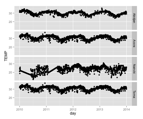

dailyMax

We can see that the Nairobi weather station is clearly missing data for 6 months of both 2010 and and 2011. The straight line is due to the linear interpolation performed in the prior step.

weatheR package

Michael Piccirilli

12/28/2014